Modeling the Rolling Shutter Effect

The Rolling Shutter Effect

Some years back, I saw a pair of excellent blog posts on the rolling shutter effect (here and here). The rolling shutter effect is a form of distortion that can appear in photographs taken on a phone, since phone cameras typically capture frames by scanning across a scene horizontally or vertically over a period of time instead of capturing the entire scene at the same instant.

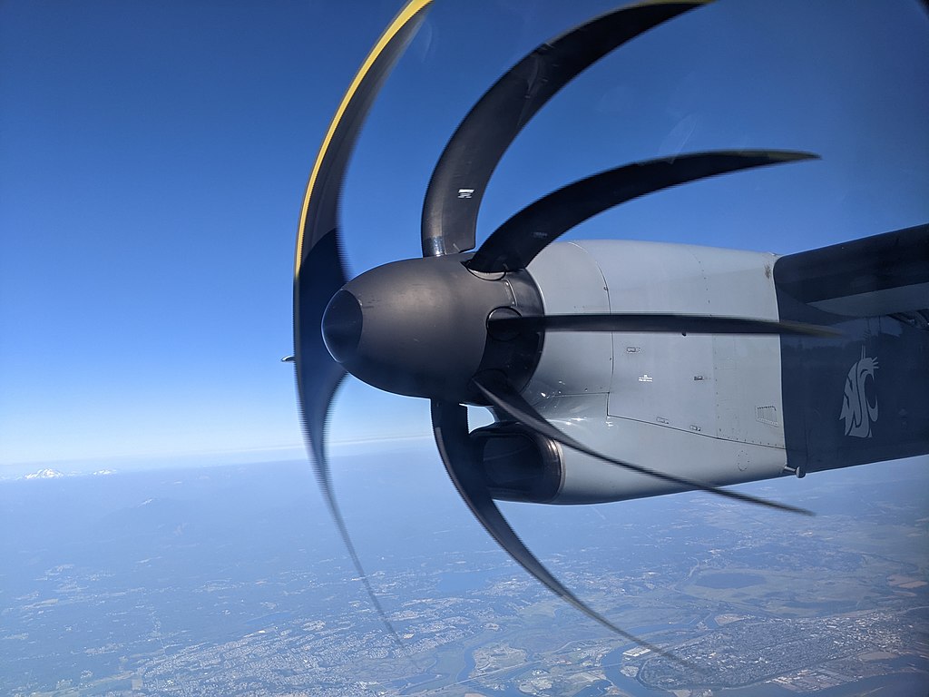
When the subject of the photograph is static or slow-moving, this method of recording an image does not cause a problem. But for a fast-moving object such as an airplane propeller, a rolling shutter can produce fascinating forms of distortion. For example, here's an image of an airplane propeller captured by a Pixel 3:

Starting with a Propeller

In order to model the effect, I started with a plot of an "airplane propeller." I used the polar equation $r = 3\cos(5\theta)$:

PolarPlot[3 Cos[5 θ], {θ, 0, 2 Pi}, ImageSize -> 300]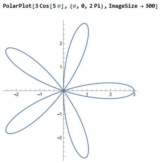

Now we can make the propeller spin by writing $r = 3\cos(5(\theta + t))$ for some parameter $t$ representing time:

Manipulate[
  PolarPlot[3 Cos[5 (θ + time)], {θ, 0, 2 Pi},
    PlotPoints -> 50, PlotRange -> {{-3, 3}, {-3, 3}},
    ImageSize -> 300],
  {time, 0, 2 Pi}, ControlPlacement -> Top]

Adding the Rolling Shutter

Next, let's get the rolling shutter into the mix. We'll start with a horizontal line at $y = 3$ that moves down as time progresses. This can be written as $y = 3 - t$. We will also adjust our propeller equation to be $r = 3\cos\!\left(5\!\left(\theta + \frac{t}{s}\right)\right)$. The newly introduced $s$ is a factor that represents the fact that the rate at which the shutter moves may differ from the rate at which the propeller rotates. We are putting the $s$ with the propeller since we are treating the speed of our rolling shutter as a constant while the speed of the propeller may vary:

Manipulate[
  Show[
    PolarPlot[3 Cos[5 (θ + time/s)], {θ, 0, 2 Pi},
      PlotPoints -> 50, PlotRange -> {{-3, 3}, {-3, 3}}],
    Graphics[Line[{{-3, 3 - time}, {3, 3 - time}}]],
    ImageSize -> 250],
  {time, 0, 6}, {{s, 1.05}, .5, 2}, ControlPlacement -> Top]

Switching to Contour Plots

In order to simulate the rolling shutter effect, it will be helpful to switch to a Cartesian plot instead of a polar plot. First rewrite $r = 3\cos\!\left(5\!\left(\theta + \frac{t}{s}\right)\right)$ as:

Then substitute in $r = \sqrt{x^2 + y^2}$ and $\theta = \arctan(x, y)$ to get:

We can plot this using a contour plot:

Manipulate[
  ContourPlot[
    (3 Cos[5 (ArcTan[x, y] + time/s)]) / Sqrt[x^2 + y^2] == 1,
    {x, -5, 5}, {y, -5, 5}, PlotPoints -> 50,
    PlotRange -> {{-3, 3}, {-3, 3}}, ImageSize -> 250],
  {time, 0, 6}, {{s, 1.05}, .5, 2}, ControlPlacement -> Top]

The Distorted Image

Finally, we need to find the "distorted" plot that is left behind after the shutter passes. We are looking for the locus of points intersecting the shutter $y = 3 - t$. Solving for time gives us $t = 3 - y$. In polar coordinates, $y = r\sin(\theta)$, so $t = 3 - r\sin(\theta)$. In rectangular coordinates, we also substitute in $r = \sqrt{x^2 + y^2}$ and $\theta = \arctan(x, y)$.

Let's substitute all of this into our contour plot equation:

This looks like a mess, but let's plot an example for $s = 0.8$ to see if the result appears reasonable:

s = 0.8;
ContourPlot[
  (3 Cos[5 (ArcTan[x, y] +
    (3 - Sqrt[x^2 + y^2] Sin[ArcTan[x, y]]) / s)]) /
    Sqrt[x^2 + y^2] == 1,
  {x, -5, 5}, {y, -5, 5}, PlotPoints -> 50,
  PlotRange -> {{-3, 3}, {-3, 3}}]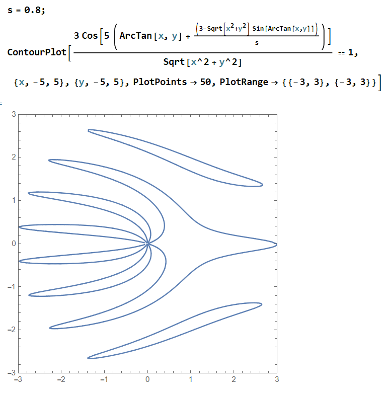

Putting It All Together

This looks exactly like the type of plot we'd expect. Let's put it all together with some better styling and optimization to make sure that the Manipulate precomputes the distorted image:

Manipulate[
  Graphics[{
    Dynamic@First@ContourPlot[
      (3 Cos[5 (ArcTan[x, y] +
        (3 - Sqrt[x^2 + y^2] Sin[ArcTan[x, y]]) / s)]) /
        Sqrt[x^2 + y^2] == 1,
      {x, -5, 5}, {y, -5, 5}, PlotPoints -> 50,
      ContourStyle -> Green,
      PlotRange -> {{-3, 3}, {-3, 3}}],
    Dynamic@First@Graphics[{Black,
      Rectangle[{-3, 3 - time}, {3, -3}]}],
    Dynamic@First@ParametricPlot[
      3 Cos[5 (θ + time/s)] {Cos[θ], Sin[θ]},
      {θ, 0, Pi}, PlotStyle -> Red,
      RegionFunction -> Function[{x, y, θ}, y < 3 - time]],
    Dynamic@First@Graphics[
      Line[{{-3, 3 - time}, {3, 3 - time}}]]},
    Axes -> False, PlotRange -> {{-3, 3}, {-3, 3}},
    Background -> Black],
  {time, 0, 6}, {{s, 0.8}, 0.3, 4},
  ControlPlacement -> Top]

Sliding the $s$ slider to the left speeds up the propeller relative to the speed of the rolling shutter, thus increasing the intensity of the effect:

Sliding the $s$ slider to the right slows down the propeller, which decreases the amount of distortion:

Mathematica Notebook

This post was originally shared on the Wolfram Community, where you can also find the interactive embedded notebook. The Wolfram Community editorial board selected it as a Staff Pick and awarded it a Featured Contributor Badge. You can view the original post and download the notebook there.